Clutter Forecast
Warning
This library is under development, none of the presented solutions are available for download.
Use continuous forest inventory databases to predict forest growth and production. Utilize traditional methods such as the Clutter model or artificial neural networks for greater flexibility. With this module, you will be able to estimate volume, the number of stems, basal area, among other variables of interest.
Class Parameters
Clutter Trainer
ClutterTrainer(df, age1, age2, ba1, ba2, site, vol, iterator=None)
| Parameters | Description |
|---|---|
| df | The dataframe containing the processed forest inventory data. |
| age1 | Name of the column containing the age of the previously sampled plot. |
| age2 | Name of the column containing the age of the subsequently sampled plot. |
| ba1 | Name of the column containing the basal area of the previously sampled plot. |
| ba2 | Name of the column containing the basal area of the subsequently sampled plot. |
| site | Name of the column containing the site index of the stand. |
| vol | Name of the column containing the volume of the subsequently sampled plot. |
| iterator | (Optional) Name of an iterator that will be used to group the data. Example of an iterator: Genetic material, Stratum. |
Example of clutter input
| Iterator | Plot | age1 | age2 | ba1 | ba2 | site | vol |
|---|---|---|---|---|---|---|---|
| GM 1 | 1 | 2.5 | 3.5 | 7.57 | 8.42 | 7.83 | 44.04 |
| GM 1 | 1 | 3.5 | 4.5 | 8.42 | 14 | 8.73 | 51.42 |
| GM 1 | 2 | 2.1 | 3.1 | 4.94 | 5.51 | 6.98 | 38.06 |
| GM 1 | 2 | 3.1 | 4.33 | 5.51 | 6.45 | 7.45 | 39.26 |
| GM 2 | 1 | 2 | 3 | 7.3 | 8.25 | 11.37 | 74.63 |
| GM 2 | 1 | 3 | 4 | 8.25 | 9.13 | 11.69 | 68.27 |
| GM 2 | 1 | 4 | 5 | 9.13 | 12.79 | 12.83 | 72.76 |
| GM 2 | 1 | 5 | 6 | 12.79 | 15.63 | 14 | 73.87 |
Class Functions
functions and parameters
ClutterTrainer.fit_model(save_dir=None)#(1)
- save_dir = Directory where the coefficients and parameters of the trained models will be saved.
| Parameters | Description |
|---|---|
| .fit_model() | Adjust the models for predicting basal area and volume. |
Clutter models
\[
\operatorname{lnb_2}^{\text{est}} =b_0 + b_1 \cdot x_1 + b_2 \cdot x_2 + b_3 \cdot x_3 + b_4 \cdot \frac{1}{I_2} + b_5 \cdot S
\]
\[
\operatorname{lnv_2} = b_0 + b_1 \cdot \frac{1}{I_2} + b_2 \cdot S + b_3 \cdot \operatorname{lnb_2}^{\text{est} }
\]
Notation
- \( β_n \): Fitted parameters
- \( I \): Age
-
\[\operatorname{x_1} = \ln(β_1) \cdot \frac{\operatorname{I_1}}{\operatorname{I}_2}\]
-
\[\operatorname{x_2} = 1 - \frac{\operatorname{I}_1}{\operatorname{I}_2}\]
-
\[\operatorname{x_3} = \left( 1 - \frac{\operatorname{I}_1}{\operatorname{I}_2} \right) \cdot \operatorname{S}\]
- \( S \): Forest site
Class Parameters
Clutter Predictor
ClutterPredictor(coefs_file, age1, site, ba1, iterator=None)
| Parameters | Description |
|---|---|
| coefs_file | Directory of the json file containing the coefficients and parameters of the fitted models. |
| age1 | Name of the column containing the age of the previously sampled plot. |
| ba1 | Name of the column containing the basal area of the previously sampled plot. |
| site | Name of the column containing the site index of the stand. |
| iterator | (Optional) Name of an iterator that will be used for predictions. |
Class Functions
functions and parameters
ClutterTrainer.get_coefs()#(1)
ClutterTrainer.predict(age2)#(2)
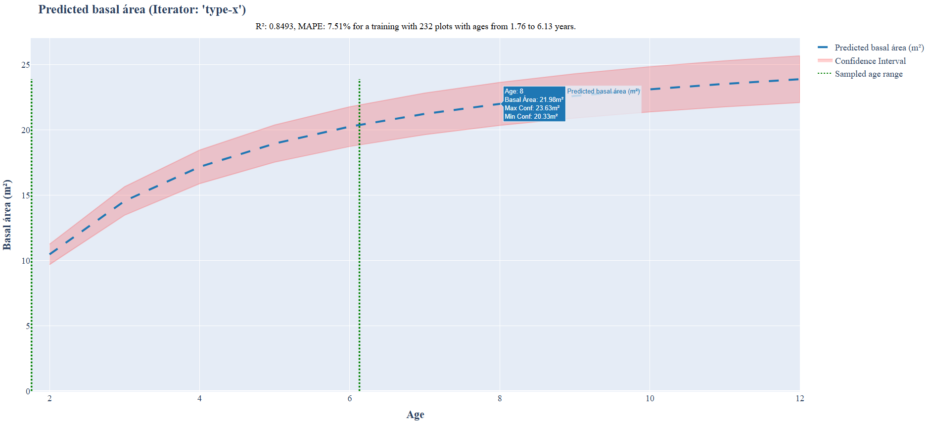
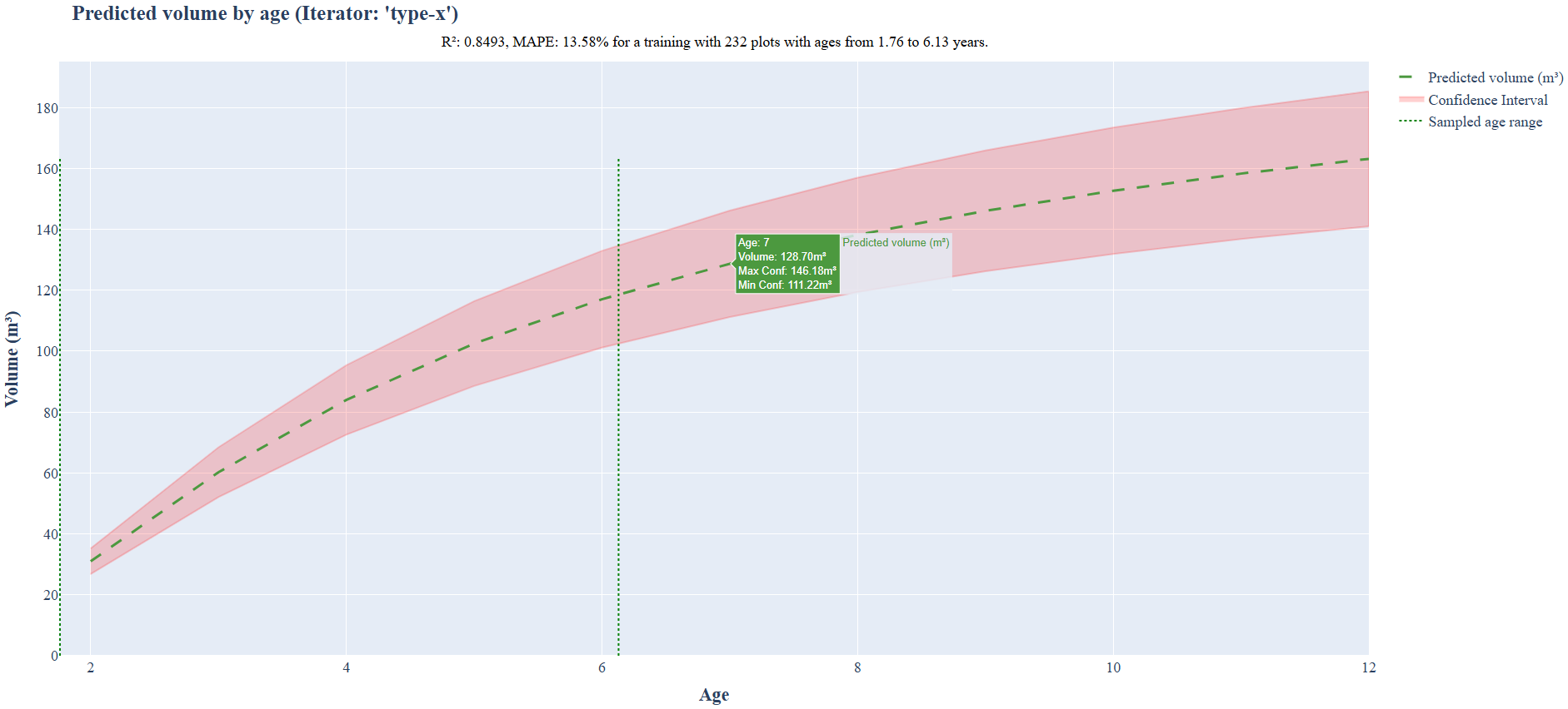
ClutterTrainer.predict_range(age_range=(2, 10),show_plots=False)#(3)
- Returns the loaded coefficients from
coefs_file. - Returns the prediction made for
age2. - Returns the prediction made for a specified age range in
age_rangeas a tuple.
Ifshow_plots=True, displays the plots of the performed predictions.
Example Usage
| clutter_forecast_example.py | |
|---|---|
1 2 | |
- Import
ClutterTrainerandClutterPredictorclass. - Import
pandasfor data manipulation.
| taper_functions_example.py | |
|---|---|
3 4 5 6 7 8 9 10 11 12 13 14 15 | |
- Load your CSV file.
- Create the variable
c_traincontaining theClutterTrainerclass. - Adjust the Clutter model, saving the coefficients and parameters in the folder
C:\Your\path\output, and save the training metrics in the variablec_train_metrics. - Create a variable containing the predictor. This predictor will use the saved model
C:\Your\path\output\all_coefficients.jsonto apply an inventory with an age of2.35, a site index of9.27, and a basal area of9.13to predict future volume production and basal area. - Make the prediction for this plantation when it reaches
4years old and save the results inba_vol_predicted. - Obtain the model coefficients and save them in the variable
coef. - Make the prediction for this plantation from
2to12years, generating a graph showing the evolution of basal area and volume over this period, along with the confidence level.
Example of output prediction plot
×
![]()